PicoScope 7 Automotive
Available for Windows, Mac, and Linux, the next evolution of our diagnostic scope software is now available.
Automotive guided tests
Library of examples on how to perform tests when using PicoScope.

Training
Our collection of training videos, articles, guides and information on training courses.

Waveform library
The Waveform Library is a global database of waveforms uploaded by PicoScope users.

Case studies
Real-life case studies show how the professionals use PicoScope to diagnose vehicle faults.

A to Z of PicoScope
Detailed description of various PicoScope software and hardware features.

Videos
Training resources and demonstrations on PicoScope and the Automotive Diagnostics Kit.

Newsletter
Archive of our monthly Automotive Newsletters.

Documentation
Download manuals, brochures, posters, and training materials.

Reviews and awards
Accolades for the preferred diagnostic tool for service centers and vehicle manufacturers.

| Vehicle details: | Mazda 3 |
| Engine code: | SH (Skyactive-D) |
| Year: | 2015 |
| Symptom: | U0100, U0131, U0151, U0155, U0214, U0415 |
| Author: | Ben Martins |
I was recently presented with a 2015 Mazda 3 with all warning lights on the dash illuminated, accompanied with around 40 DTCs (diagnostic trouble codes). As with anything slightly out of the ordinary, the customer interview is vitally important to get an idea of what is going on and when it all started and, normally, this helps give you some direction. That was not the case with this one.
I was informed that this was an intermittent fault (a personal favourite of mine) that may happen within the first 50 or 300 miles of driving. When the fault occurred, the RPM needle would drop to 0 and then the dash would light up. The RPM gauge would return but the lights would stay on, and once the ignition was turned off and on again, the lights would extinguish until the next time the fault occurred. As I delved deeper into the history of the vehicle, I also learned that the ECUs for the ABS, SAS (SRS), Start Stop and FBCM (Front Body Control Module) had been replaced and to add even more to mix, the vehicle had also been involved in an accident on the OSF (offside front) of the vehicle.
As the warning lights were present already, I did a quick DTC scan which revealed a massive amount of DTCs. With this many fault codes present, it was very difficult to get any sort of direction. To name a few: U0131, U0151, U0155, U0415, U0100, U0214. All of these are communication fault codes that report the loss of an ECU on the network.
So, where to start with this many faults? With a reasonably large amount of information to take in it’s always good to look back over the information gained from the customer to try and build a picture of the situation.
From the numerous fault codes and the fact that ECUs were reporting the loss of another ECU I could take an educated guess and say that what we were looking at was a network failure of some description. However, before I started any diagnosis, it was vital to understand how the system worked. By referring to my knowledge and a wiring diagram I could start building a picture of how the network operates and where each ECU is along the line.
From the wiring diagram, you can see which ECUs should be seen on the high-speed CAN line. There are now a number of different configurations given to a network, so a detailed wiring diagram is essential. Given the position of the diagnostic port on the network, we attempted to talk to all the ECUs along the network. From the initial global scan from the diagnostic tool we could see and access live data, so at that moment in time, the network was ok. However, while we were looking at the PCM, communication dropped out and I was unable to re-establish it. Great! With anything intermittent getting it to replicate the symptom described by the customer can often be the hardest part.
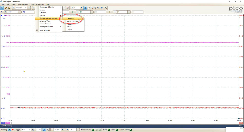
Now I wanted to take a look at what the CAN H & L signals were doing. Connecting PicoScope is a quick and easy way to check the signal for correct pattern. By using the dropdown menu on the automotive tab, you can select the CAN H & L Guided Test. It will provide the settings for the test, with a reference to what the pattern should look like and information on how to connect.
One of the biggest problems you can face when capturing CAN faults is the speed at which they happen. Currently, we just wanted to get an idea of what was going on, so the more data we could get the easier it would be to see on the screen. If you increase the waveform buffer the scope will record for longer. To do this, go to Tools > Preferences and increase the maximum number of waveforms. In this first instance, the details weren’t as important as capturing the fault as it happened.
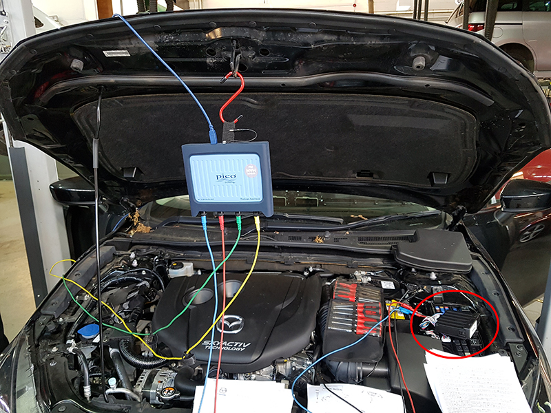
So where should you test? Removing as little as possible is always best as time is often against us. As I was still connected to the scan tool through the 16-pin port, I had to find an easily accessible point to access the network through. I could have used the 16-pin breakout box, but I felt it was important to check further away and, more importantly, I didn’t have one with me. Referring back to the wiring diagram, the FBCM (front body control module) would seem a good starting place. It links the ABS ECU and PCM to the rest of the CAN network and as luck would have it, it had an easy access point under the bonnet.
Again, you must always refer back to the wiring diagram for confirmation of correct pin numbers and ECU locations. The initial findings for the CAN line were good, however, there was a very odd spike which wasn’t completely captured as it over ranged. For a CAN line, that is not normal. A normally operating CAN High signal usually has a range between 2.5 V and 3.5 V.
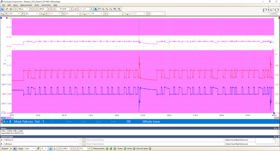
By using the math channel and mask features in PicoScope, I could quickly visualize problems across the whole capture. The inbuilt A + B math channel gives the total of the CAN H and CAN L signal and could highlight any slight anomaly. Adding the two channels together should always give a 5 V constant, therefore, anything outside of this can be regarded as abnormal. By including a mask, (see figure 7), you can easily see the area of concern as anything outside of a specified value is obvious.
For further information regarding masks in CAN please visit the link to the forum page Trigger from math channel? or alternatively, see page 175 of the PicoScope 6 User’s Guide.
Taking into account that there was a slight discrepancy with the signal and that the vehicle had been involved in an accident OSF, I felt it best to make sure that the wiring around this area was ok. I referred to the wiring diagram again, confirming that there were a number of earth points sitting in this area. Too often you find that the body shop has removed the wiring, painted over the contact point and re-fixed it. This will inevitably cause grounding issues from poor contact. Without having to remove too much I was able to inspect the ground points and found the wiring to be in a good condition.
So I went back to the wiring diagram. The next step was to carry out a comparison of the signal between two points on the network. The reason for this being that the majority of the codes referred to a loss of communication between ECUs. If you look at two relatively accessible points you will be able to see if the data packets are being sent at the same time or if there is a breakdown in the communication. The instrument cluster is at the end of the line and contains the terminating resistor. It was relatively straightforward to get to and there was a handy junction connector that meant I could get to the wiring without having to disconnect the instrument cluster. However, as nice as it would have been to get to the PCM connector, it was protected by shear bolts and a rather large piece of metal so I decided it was best to stay connected at the FBCM.
I now had all four channels monitoring the CAN H & L signals at two separate points on the network (figure 9). Number 1 is on the FBCM which represents channel A and B on the scope and Number 2 is on the junction connector joining the instrument cluster which is channel C and D on the scope. With the car ignition on, we can see what is happening to the network making it lose communication.
I kept the previously mentioned math channel and included another one to measure C + D. The initial pattern seemed ok but then it quickly started to deteriorate.

Figure 10
In Figure 10 you can see the CAN H & L signal from FBCM at 1 and at 2 taken from behind the instrument cluster.
As the scope continued to capture over time, it became quite clear that something was not right. As you can see in Figure 11, there is a now a problem. The two CAN signals, which were on the same line, no longer matched up.

Figure 11
PicoScope also has a function that allows you to decode serial information. To see the physical layer cleaned up I had to create another math channel: A – B. (It is important to make sure that you have Channel A as CAN H and Channel B as CAN L. If it is the other way around, the calculation will not work and the channels would need to be reversed to display it correctly.) This will enable the serial decoder to give a true representation of the data packet. For more information regarding CAN serial decoding, please visit our forum post CAN decoding in color.
However, I still did not know where the data had come from or where it was going. What you can see, are the ID codes for the data packets (see figure 11, marks 3 and 4). These should be the same at each end of the network. Clearly, from figure 11, this is not the case. At this stage, I decided to stop and take note of what I had seen so far.
Back to the wiring diagram. This is where access to a good wiring diagram is important. From the diagrams I had access to, I found something very interesting. Most manufacturers will put junction blocks into the network to link all the various ECUs together. This can be particularly useful if one ECU has shorted, causing a communication issue. By simply disconnecting a junction block, the offending section of a network, and subsequently the offending ECU, can be isolated quickly. On a good diagram you will normally have the locations for the various connectors and as before there is a case of hunting down the fault without having to strip the vehicle. By looking at the diagram I could begin to narrow down possibilities and find where to look next. What became clear from the diagram was that there were four distinct points where the network passed through. Time to start resistance checking.

Figure 12
Finding the locations of these junction connectors can sometimes be tricky as they’re not always in the easiest of places to get to. Picking out the easy to access points is always going to be first on my list. I saw that Junction block number 2 and the front camera connector were located on the NSF of the cabin and found it best to start there. I removed the glovebox which gave me good access. The junction blocks also help when resistance checking as you can eliminate parts of the circuit very quickly. As the instrument cluster was already out it seemed logical to start there and make my way down the line. Everything checked out fine. 0.2 Ω measured with no short to ground or to each other. My hope was fading fast as the other plugs were not so easily accessible.
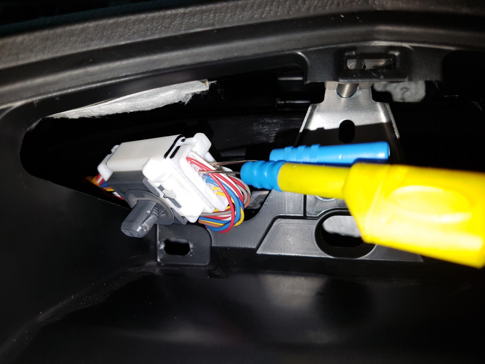
Then, a breakthrough! I removed the A-pillar trim on the NSF which revealed the front camera connector for the roof wiring. What we found was quite surprising, to say the least, but made perfect sense.

Figure 13
The plug was not fully connected. It turned out that the wiring for the safety camera was a loop in the CAN network, which meant that as soon as the plug lost contact, it would split the network in two. So while the connection was good sometimes, any slight bump in the road, temperature change or body flex would cause the circuit to break. This would explain the difference in data packets, the odd spikes of voltage PicoScope was picking up and the vast range of fault codes reporting a loss of ECU’s. While I was there it felt right to make sure that the wiring was conforming. A quick check; from the connector, down the junction block behind the glove box and then down to the FBCM, made me fairly confident that the wiring was ok. I reconnected the plug, made sure it was secure and cleared the fault codes. I then looked at the data again from the same two points, FBCM and the junction connector behind the instrument cluster.

Figure 14
Now as you can see it all matched perfectly and the H and L signals are mirroring each other as they should. There is still this odd spike at the end of the data packet, but this is a characteristic of the End-Of-Message part to the data packet. To be confident that this insecure plug really was the source of the issue, I decided to check by disconnecting it again and see what happened. Sure enough, the data goes all over the place. Misplaced data packets, warning lights, RPM signal on instrument cluster dropping and all the DTCs that were there previously returned. As this was an intermittent fault, the only thing left to do was to test it. Normally I would have kept the vehicle and done some extended road tests to make sure that the problem was fixed permanently, but logistically this was not an option.
To sum up this case: The vehicle had numerous warning lights intermittently, along with numerous DTCs relating to communication faults. By looking at the signal on PicoScope, I confirmed communication faults by using masks and math channels. The correct detailed wiring diagrams were essential in understanding how the network was connected. I found a direct link to the faults and confirmed the diagnosis by re-introducing the fault to check that I had the same faults and symptoms.
My advice regarding CAN or network faults is to never give up. There is always a solution. I believe it is important not to be afraid of CAN or network faults. Over the years I’ve seen many a technician get very nervous about the thought of doing any diagnosis of network faults, but essentially we are just looking at voltage. This is where the scope has become a vital piece of the diagnostic puzzle as it gives us the ability to see voltage over time, something you would not be able to do with a multimeter.
John
December 11 2021
You fancy fixing my car
Jahn deaux
January 16 2018
I do essentially the types of diagnostics you detailed in this case study, and usually not the first but certainly the last. I like the challenge, but as we all know the intermittents are the most difficult diagnostics. Good job. These case studies are quite informative. I am a fan of scope and the Pico in particular.
Steve Ashcroft
September 24 2017
Thank You, a very good case study as I have just spent hours on a can fault on a Citreon DS3!
Robert Squibb
September 02 2017
An excellent and very informative article, explaining a very logical and methodical diagnosis! Thanks.
Dean C
September 02 2017
Very nice job! It’s always good to see post of this kind on network problems.
Simon Mcloughlin
August 31 2017
A very good write up on real world use of the diagnostic equipment and your approach to break it down and isolate it. Well done.