PicoScope 7 Automotive
Available for Windows, Mac, and Linux, the next evolution of our diagnostic scope software is now available.
Automotive guided tests
Library of examples on how to perform tests when using PicoScope.

Training
Our collection of training videos, articles, guides and information on training courses.

Waveform library
The Waveform Library is a global database of waveforms uploaded by PicoScope users.

Case studies
Real-life case studies show how the professionals use PicoScope to diagnose vehicle faults.

A to Z of PicoScope
Detailed description of various PicoScope software and hardware features.

Videos
Training resources and demonstrations on PicoScope and the Automotive Diagnostics Kit.

Newsletter
Archive of our monthly Automotive Newsletters.

Documentation
Download manuals, brochures, posters, and training materials.

Reviews and awards
Accolades for the preferred diagnostic tool for service centers and vehicle manufacturers.

Filtering: When, Where, Why and How?
A video supporting this Guided Test and the supporting PSDATA file can be found at the bottom of this page.
In this article, you will discover a number of PicoScope features and techniques that will reveal the signal that lies beneath. In this typical example, we are using a narrowband Zirconia lambda sensor.
Both the test procedure to capture this waveform, and the expected result from the capture of such a component has been well documented in the past. With its characteristic sine waveform switching from 0.1 V to 0.9 V at a frequency of 1 Hz (see the Guided Test menu within your PicoScope software: Automotive > Sensors > Lambda > Zirconia).
 |
What is not so documented is the vulnerability of such a signal in the harsh environment of the engine bay, with high frequency switching components radiating EMI (Electromagnetic Interference). The image above presents a typical example of noise induced into a lambda sensor signal, seen here as long rising a falling spikes and hash about the sine wave that lies beneath.
The quality of tool used to capture the lambda sensor signal will determine just how much of this noise is visible. Many budget tools have a low bandwidth and so cannot pick up high frequency noise. Ironically, this characteristic will benefit signals such as those from a lambda sensor, but will fall short for signals such as CAN, injection and ignition. Tools such as these will present a textbook artificially conditioned signal to the technician revealing only half the story!
Could the noise actually be responsible for a lambda sensor code or an emission failure? Within the noise itself could be evidence of ignition/injection spikes, arcing from worn components, chaffing to adjacent cables or internal shorting in the lambda sensor heater element / engine ground.
Without the true signal revealed on screen, how will we ever know?
Fundamentally, unpowered sensors such as lambda have a high output resistance leaving both the sensor and wiring prone to the pick-up of noise. Inside the PCM the signal will be filtered but it is vital to see both the unfiltered and filtered version as the comparison will help to reveal what is expected noise and what is affecting the signal as seen by the PCM.
There is a phrase mentioned here at Pico that refers to any data acquisition and that is, "catch it dirty" which means the signal you see on screen is a true representation of the actual signal with no conditioning. With this data technicians can evaluate the noise and then implement a number of the PicoScope features at their disposal to clean and filter the signal into something viable.
Before diving into filtering (reducing signal noise) we must ensure our PicoScope is connected to out PC/Laptop using the Pico Blue USB cable and NOT a generic USB cable. The Pico Blue USB cable has quality assured termination at each plug, improved grounding and a superior wire core to ensure minimal power loss, excellent data transfer and true grounding. Be aware of poor quality aftermarket laptop chargers as these have the potential to introduce noise.
Both the PicoScope itself and the test leads we provide are well screened to avoid the pick-up of noise, the same however cannot be said of the vehicle wiring harness. In the average vehicle, few signals are screened (to reduce costs) and sensitive signal wires are often run next to cables carrying signals that radiate noise such as those used for injectors.
Unscreened wires in the engine bay have the potential to pick-up noise from other noisy sources such as some overhead lights, electric lift motors, welders and overhead power cables etc. It is cheaper for vehicle manufacturers to use unscreened cables and then filter out the noise inside the PCM than it is to use nicely screened cables! Therefore, this makes our job more difficult as we have to work out what is normal noise and what is abnormal.
Assuming all the above have been considered and in place, we now have a multitude of options to filter notorious signals such as lambda sensors.
Let's start at the beginning, before capture!
Ground reference measurement
The test lead ground cable must be connected to the battery negative terminal. This is due to the fact that we measure our signals with reference to vehicle ground when using a PicoScope with common ground BNCs (where all BNC terminal grounds are connected to one another, such as the PicoScope 4423, 4223, 3423 and 3223).

Differential measurement
When measuring sensor signals (such as lambda) with the new PicoScope 4425 or PicoScope 4225 the option to connect our test lead ground cable to the lambda sensor ground wire is available, and often helps to reduce noise on our signal. Here we have a differential measurement utilizing the lambda sensor ground, which is partially shielded from such EMI (via the PCM) so producing a cleaner signal.

 |
 |
||
| Acceptable lambda sensor connection for all PicoScopes: Ground reference measurement |
Optional Lambda sensor connection for PicoScope 4425 and 4225 only: Differential measurement |
Hardware Filter
For those lucky enough to be using the new PicoScope 4225 and 4425 models there is an additional line of defense from high-frequency noise in the form of a Hardware filter (bandwidth limiter) that is a setting applied prior to capture.
This filter will reject all noise above 20 kHz before the signal is passed through to the scope for processing. In effect, we convert the selected scope channel bandwidth from 20 MHz to 20 kHz
The advantage of using the hardware filter is that it allows you to use a lower input range to capture the signal.
Think of a lambda sensor where the signal voltage of interest is 0.1 V to 0.9 V yet the noise present may exceed 50 V. Selecting a 50 V scale in order to encompass the noise will result in poor resolution of our 0.1 V to 0.9 V signal. With the bandwidth limiter active, we concentrate only on the signal range we are interested in.
There is a good argument for leaving the hardware filter on indefinitely for most automotive signals (other than those where high-frequency noise measurements are required, such as CAN, FlexRay and some ignition/injection captures). This is especially true for current clamps as they do not detect signals over 20 kHz which is too high a frequency to be hiding any issues of concern (maximum current clamp bandwidth is 20 kHz).

Activating the Hardware Filter
With a PicoScope 4225 or 4425 connected, select Tools > Preferences > Options > and check the box marked Show Analog Options followed by OK. This will allow for the Hardware Filter to be activated within the Channel options menu and limit the bandwidth to 20 kHz for all incoming signals of your chosen channel.
A word to the wise about using the Hardware Filter:
The hardware filter cannot be switched off after capture to reveal the original signal. Unlike software filters such as low pass filter and math channels that can be applied or removed after capture.
The examples below were captured using the Zirconia Lambda Sensor Guided Test:
 |
 |
|
| Lambda signal without Hardware Filter | Lambda signal with Hardware Filter |
<td style="text-align: center;">Lambda signal without Hardware Filter</td>
Here we have immediately quenched some of the high-frequency noise (above 20 kHz) before it enters the PicoScope. Remember: the Hardware filter is only relevant to users of the new PicoScope 4225 and 4425 models and so from here on in, everything written below is relevant to all PicoScopes.
Software Filters (Low Pass using Channel options or Low Pass using Math Channels)
Like any measurement, it is essential to ensure we have the correct settings such as Voltage range, Timebase and the relevant number of samples across the screen (500 kS minimum).
It may be tempting to go for a ±1 V scale for a signal from 0.1 to 0.9 V, however, noise levels are likely to exceed this limited voltage range (voltage spikes will often exceed 20 V!). For this reason select a voltage scale of ±20 V.
It is important for PicoScope to keep all the noise present on our signal within the voltage range of the scope in order to successfully apply a filtering math channel later on. Our Math Channel filter option works by taking voltage values at thousands of point across the entire waveform and bases calculations on them. Should an over-range occur (in the case of a 20 V spike on a ±1 V scale) the Math Channel attempts to apply a filter to an infinite value (over-range), producing an erroneous waveform.
Given we have selected a ±20 V scale for what is in effect a 1 V signal, adjust the vertical zoom feature by a factor of 5 (x5) so you have a ±4 V range. Now we have the best of both worlds with better resolution of our 1 V signal, whilst preventing an over-range condition due to voltage spikes.
 |
Activate the Low Pass filtering option from the channel option menu
This filter style has the advantage of being quick and easy to use whilst allowing varying levels of low pass filtering to be applied whilst monitoring the effects of the filter upon the captured waveform. Be aware of over filtering as the original waveform can become unrecognizable!
Remember low pass filtering (using the channel option menu) can be applied after capture and so can be used not only during diagnosis but when reviewing captures of saved waveforms away from the turmoil of the workshop.
Click on the relevant Channel options (1) button to reveal the LowPass Filtering check box. Place a tick in the checkbox (2) and ensure a 100 Hz Low Pass filter is applied to the input signal.
Below, 100 Hz is chosen as the desired level of low pass filtering for our example lambda sensor:
 |
The disadvantage of this style of filter is that we cannot filter live at slow time frames (streaming mode) unlike the Hardware Filter, and so we are required to halt our capture, and then view the filtered waveform by scrolling through the waveform buffer
Activate a hidden feature called Display Last Waveform that will enable the filtered waveform to remain on screen whilst PicoScope draws the new waveform alongside. This will allow the technician to view sensor operation continually on screen rather than waiting for the live waveform to be drawn before the scope momentarily displays the filtered signal. The technician will now have a continual view of the filtered signal without having to stop the capture and scroll through the waveform buffer.
Select Tools > Preferences > Sampling > and check the box marked Display previous Waveform Buffer.
Below we can see the Display Previous Waveform Buffer feature in action with our filtered and unfiltered signal visible. The new “live” unfiltered waveform (left) accompanied with the filtered previous waveform (right).
 |
An alternative to the Low Pass filtering available in the Channel options menu is the Math channel option.
Implement low pass filtering using a math channel
Whilst this filter style will take longer to set up initially, it has the distinct advantage of allowing both the filtered and unfiltered waveform to be viewed at the same time and once created will remain in your maths channel library ready for use whenever required (create once only).
Before creating a low pass maths channel, turn off the low pass filter and display previous waveform buffer features above. Now you should be running a non-filtered lambda sensor signal
(20 V scale x 5 vertical zoom 500 ms/div, no filter and display previous waveform buffer set to off).
Creating a maths channel incorporating a 100 Hz Low pass filter will create a reproduction of your sensor signal but with all the high-frequency noise (above 100 Hz) removed. Only lower frequencies below 100 Hz will be allowed to pass.
This is a very simple process and once created can be saved in your maths channel library for use with future signal measurements such as lambda.
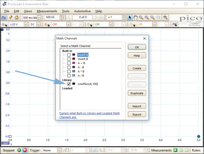
Select Tools > Math channels > Create > Next > Advanced > Filters > and click on the Low Pass symbol.
The title “LowPass ()” will appear in the formula box. Clicking the channel letter you require will add the channel to the formula, and typing “,100” adjacent to the channel letter between the formula brackets completes the formula. The whole Math channel formula should look like “LowPass(A,100)” for a 100 Hz low pass filter to be applied to Channel A.
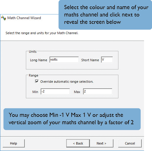
Selecting Next allows for color and name choice for your maths channel, select Next and tick the box marked Override automatic range selection. Enter a voltage range for your maths channel “-2 v to +2 V” select Next and click Finish. Check the box of your newly created maths channel in order to display the filtered signal of your original capture.

The settings are now complete to capture the original lambda sensor signal accompanied with the added filtered maths channel so allowing the technician to monitor the filtered and unfiltered signals.
 |
Once again, low pass filtering (using a math channel) can be applied post capture and so can be used not only during diagnosis but when reviewing captures of saved waveforms away from the turmoil of the workshop. Whilst the maths channel serves as an alternative filter for lambda sensor signals, the benefits are more appreciable when used in conjunction with higher frequency sensors such as crankshaft sensors, where you may wish to remove high frequency ignition noise. A typical example formula would be LowPass(A,5000) for a 5 kHz low pass applied to a crankshaft signal on Channel A.
 |
 |
|
| Original Lambda sensor signal | Signal with filtering applied |
The test process and information above serve as a guide only, and are not necessary for every sensor. As your experience with PicoScope grows, you may find that simply activating Lowpass Filtering (via channel options) with a ±2 V range is sufficient for what you require from your captured signal.