Maths is cool - part 1
by Steve Smith

In this educational series, Steve Smith shares his knowledge about using math channels in PicoScope. The series covers why the math channels in PicoScope are so useful and how to use them for applications like calculating resistance, power, rpm, torque, voltage drop, etc. As Steve says: I wanted to write about the power of maths. There I so much that can be revealed by applying math channels to the raw data that has been captured. The real beauty of math channels is that they are applied post-capture to existing and already saved files that may be years old to reveal new information about past faults. Maths is cool! 

For more information about how you access the math channel menu/wizard, this and the in-built math channel A-B is discussed in the Scope School Extra - Bonus Class.

The application of math channels:

1. Make sure that you have enough samples on the screen, ideally a minimum of one million.
2. Make sure you have sufficient data on the screen containing the relevant information required, e.g. voltage fluctuations or a number of specific cycles/events.
3. Give PicoScope the time to fill the screen with data, do not stop the capture midway across the screen.
4. Make sure that the captured signal does not over-range at any point during the capture.
5. You may have to apply lowpass filtering to remove noise/spikes from the waveform. This will even out the math channel equal to the original signal.

Example of typical waveform ideal for use with math channels:

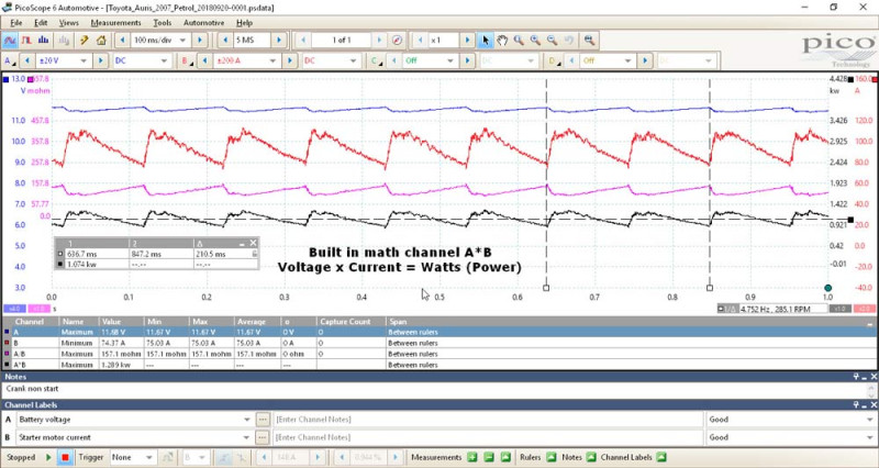
This waveform consists of the battery voltage and the starter motor current on a cranking, engine during a relative compression test. It has sufficient samples, a complete screen/buffer of data with a number of compression events and with no over-ranging. It has a 1 kHz lowpass filter applied to Channel A and B in order to improve the results displayed by the math channels.

Starting with the math channel A/B (voltage divided by current), we can display the circuit resistance during cranking. Note how the resistance decreases in proportion to the current flow through the starter motor during each compression event (Ohm’s law in action).

Now, if we multiply Channel A with Channel B (voltage*current) we get Watts (power) where the peak electrical power occurs at peak compression, measuring approximately 1.28 kW.

Knowing the number of cylinders for this engine, four, we can determine the frequency of 2 x peak compression events based on peak current. These are evident between the time rulers.

A four stroke, 4-cylinder engine will produce two compression events per engine revolution. If we know the frequency of these events, we multiply by 60 to obtain and graph RPM (cranking speed as indicated in the Frequency/RPM legend).

The formula for RPM is, in this scenario, 60/2*freq(B). Notice the excellent and stable cranking speed of approximately 280 RPM across the whole capture.

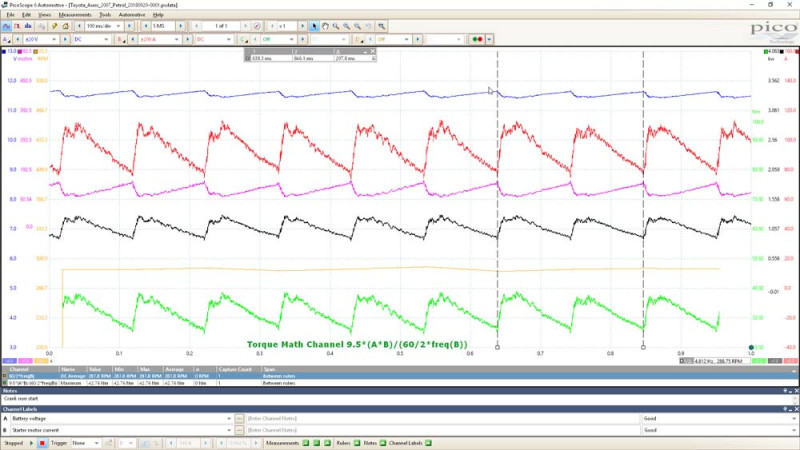
Finally, we can also obtain torque. Given that we know power and RPM, add in a constant of 95 (for Nm) and this is the formula: 9.5*(A*B)/(60/2*freq(B)).

The waveform in figure X shows how peak torque occurs at peak compression, using Channel B – current as our reference.

We originally started with a simple capture with only voltage and current but with the addition of some maths, now we also have resistance, power, speed and torque.

The PicoScope file below contains all the waveforms and math channels used in this session. Remember to activate the lowpass filter for Channels A and B.

Toyota Auris 2007 petrol.psdata